Nelson Winter Model of Industrial Dynamics
Contents
Introduction
Nelson and Winter have developed the most influential simulation models to analyze the processes of industrial dynamics and economic growth. Their models are perfect examples of the KISS principle in simulation. The models and the evolutionary theory on which the models are based are explained in detail in their path-breaking book, Nelson, R.R., and Winter, S.G. (1982), An Evolutionary Theory of Economic Change, Belknap Press, Cambridge, Mass. and London.
This site provides a simple implementation of the basic industry dynamics model in spreadsheets and R so that anybody without a programming knowledge can “play” with the model, run different experiments, and get the feeling of micro-simulation modeling. All the models presented on this web page are freely available for non-profit research and education. Please feel free to copy and redistribute them in modified or unmodified form.
Java and LSD implementations of similar models are available on Murat Yıldızoğlulu’s and Esben Sloth Andersen’s web pages, respectively.
For comments and questions, please contact Erol Taymaz.
Base model
Nelson Winter Base Model is based on the model presented in Nelson and Winter’s book (An Evolutionary Theory of Economic Change) in Chapter 12. Firms spend a constant amount of money on innovative and imitative R&D activities. More productive firms (thanks to innovation and imitation) become more profitable, make more investment, grow faster, and, consequently, increase their market shares. However, because of the fact that innovation and imitation are random processes in which the probability of innovation and imitation depends on R&D expenditures, there could be shake-ups in market shares. There is no entry and exit in the base model.
Spreadsheet Version of the Base Model is available in Open Office (320 KB) and Excel/XP (610 KB) formats.
The Nelson-Winter Base Model (Spreadsheet Version) is written in various self-explanatory sheets. The first sheet, Parameters, includes the parameters of the model. Users can easily change parameter values to run different experiments. Once a parameter value is entered, all sheets are automatically calculated, and a simulation result is obtained. If the user presses “F9” (re-calculate), all sheets will be re-calculated, that is, a new experiment with the same parameter values will be run. Therefore, the users can keep pressing the F9 key to see the effects of stochastic factors (innovation and imitation) in the model.
The second sheet, K, contains the capital variable. At the beginning of simulation, all firms have the same size (capital stock). Capital stock each year is updated by investment and depreciation.
The third sheet, A, keeps the level of productivity, which is the same for all firms at the beginning. Productivity increases to a level randomly determined from a uniform distribution between the existing level and the frontier level if the firm innovates or between the existing level and the level of the most productive firm if it imitates.
The fourth sheet, Q, is output and calculated as K*A.
The Profit is calculated as profit per capital. The profit of the firm is equal to total revenue minus “cost of capital” minus innovation expenditures minus imitation expenditures. In the current model, the last three are taken as user-defined parameters, and are same for all firms.
InnDraw and ImmDraw are innovation and imitation draws, respectively, and show if the firm innovates or imitates. Innovation and imitation are determined randomly, and their probabilities depend on innovation/imitation expenditures (and exogenous parameters that can be changed by the user).
The next sheet, s, keeps the data on market shares. It is used to draw the chart for market shares.
The last variable is investment, _Invest. Investment level depends on the firm’s profits and borrowing from the bank.
Finally, there are some charts to visualize experiment results. They depict productivity levels (_ProdLevel), concentration level in the market (Herfindahl index, _Concent), market shares (_MShare), total quantity supplied (_Q), and the product price (_Price).
R version
R Version of the base model__ is available as an R script file (only 7.1 KB).
R is a great free software environment for matrix operations, statistical computing and graphics. It compiles and runs on a wide variety of platforms (Linux, Windows and MacOS). You can get the latest version freely from the R-Project web page. Although it is not essential, it makes to run programs much easier if you use an integrated development environment (IDE) for R. There are many alternatives, and I could recommend RStudio. RStudio is also a great free software and is available for all major platforms including Linux, Windows, and MacOS.
The Nelson-Winter Base Model (R Version) is composed of various functions. In order to run the program, first open the R program, then read the script file (NW_BaseModel.R) by the “source” function. When the script file is read, all functions will be ready. Alternatively, if you use an IDE (like RStudio), open the script file, and run all lines.
The following functions are available in the NW_BaseModel.R script.
run() is the main function that runs the model. It may have three arguments: nIter (number of iterations), nFirm (number of firms) and setSeed (setting the initial seed). The default values are nIter=100, nFirm=8, setSeed=FALSE. In other words, if you simply type,
run()
the model will be run for 100 periods for 8 firms, and the initial seed for pseduo-random number generator will use the value it has when the function is run. If you would like to run the model longer (let us say, 500 periods) with more firms, you may type run(500, 10, TRUE)
If you set setSeed value to “TRUE”, then the initial seed value for the pseude-random number generator will be equal to 123 (you can change that value to any other one by modifying the “setPara” function). Setting the seed number will guarantee that you can replicate the same simulation anytime you like.
The run() function calls all other functions required to run the program. iterate() is the function that runs the model for one period.
The setPara() function sets parameter values. You can change all parameter values by modifying this function.
The setFirms() and setMarket() functions initialize firms and markets, respectively.
The invest() function calculates the investment level for each firm. innDraw() and immDraw() are innovation and imitation draw functions, respectively.
pMarket() plots four charts about the market outcomes: product price, concentration level, maximum technology (technological frontier) and average technology level. When you run the model, pMarket() function is called by the run() function at the end of simulation, and all these charts are plotted in one page. If you would like to get charts on firm-specific variables, you may use pMS() function that plots markets shares of all firms, and pTech() function that plots technological levels of all firms. pAccum() function plots four charts that help to understand the dynamics of capital accumulation: growth rate of aggregate output, growth rate of aggregate capital stock, average profit rate, and average investment intensity (aggregate investment/capital stock ratio). To summarize, you can simply type
run(xx, yy, TRUE)
to simulate the model for xx periods for yy number of firms. In order to test the effects of random factors, run the same simulation by changing the initial seed as follows:
run(xx, yy, FALSE)
Entry-exit model
The Nelson Winter Entry-Exit Model is same as the Base Model, but now we allow for entry and exit of firms. The number of entrants increases by the profitability of the market, and those firms that cannot achieve “satisficing” level of profits will exit. Because of the (endogenous) changes in the number of firms, spreadsheets are not suitable tools for these model. Thus, we use R to model the Nelson Wintor Entry Model.
The Nelson Winter Entry Model includes all functions available in the base model. It has two additional functions: enterFirms() and exitFirms(). As their names imply, the first function cretaes new firms, and the second function deletes unsuccessful firms. The number of new firms depends on some exogenous parameters and the average profitability in the market. Exit depends on the number of periods with negative profit rate. The user can change parameter values so as to make entry faster and/or strongly correlated with market profitability, and to make exit faster.
R Version of the Nelson Winter Entry Model can be downloaded from here (9.2KB).
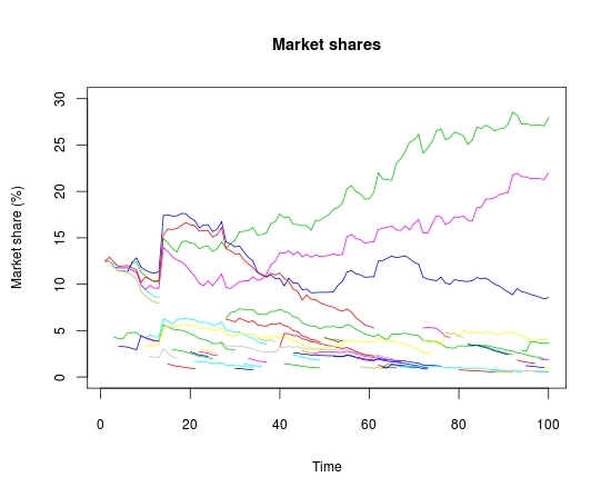
NW Model Market Shares