Lecture 4. Tutorial Cases that Come with OpenFOAM
WARNING: THIS LECTURE IS INCOMPLETE. IT IS A WORK IN PROGRESS.
As mentioned earlier in Lecture 2, OpenFOAM comes with a tutorial directory, in which there are several ready to solve problems (cases). They are
important because we can learn a lot by studying their files and solving them. Also, to solve a new problem we can find a similar one in this folder,
copy its files to a new folder and edit the files according to the needs of our problem. This is easier than creating everything from scratch.
Although this directory is called tutorials, unfortunately there are no detailed explanations of the problems. For some problems the directory names
are helpful to understand what the problems are about, but for some others you need to dig deep into the files and run and post-process the problems
to really understand what they are about. I think the learning curve of OpenFOAM could have been much more gentle, if the developers or the community
members had prepared a detailed documentation of these cases.
In version 7 of CFD Direct distribution the problems are grouped into 15 folders as shown below, with many sub-folders in most of them. In the coming
sections I will provide brief explanations of some (not all) of these problems.
The three executables seen above in green color are shell scripts that are used to perform the following tasks.
- Allrun: Performs all the necessary preprocessing (mesh creation, etc.) for all the cases (problems) and solves all of them. Running this may
take many many hours, if not days, to finish.
- Alltest: Quickly performs a test on all the cases, not actually solving them.
- Allclean: Brings the case folders to their original states, deleting created meshes, result files, etc.
You'll also find Allrun scripts in many of the individual problem folders. Using them will only solve the respective problem. The tutorials
are located in /opt/openfoam7/tutorials/ directory, for which only the users with root privileges have write access. Therefore, to solve
these problems you better copy the ones that you are interested in to your working folder using commands such as the following.
> cd
> mkdir openFoamTests
> cd openFoamTests
> cp -r $FOAM_TUTORIALS/mesh/blockMesh/pipe .
where the first command takes us into our home folder, in case we are somewhere else, the second line creates a working folder, third one goes into that
working folder and the last one copies the tutorial folder "pipe" into our working folder. Note that $FOAM_TUTORIALS is an environment variable pointing
to OpenFOAM's tutorial folder. If we check what we actually copied, we'll see one file and 2 folders.
Running the Allrun script, a mesh will be generated, because this case demonstrates the use of the blockMesh mesh generation utility.
Following is a list summarizing what some of these tutorial cases are about. To create it, I run and post-processed all of them one-by-one. As far as I know,
such a list does not appear anywhere on the web.
4.1 Tutorials in the "mesh" Folder
These demonstrate OpenFOAM's mesh generation utilities.
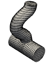 |
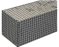
/blockMesh/pipe/
Creates the shown mesh using the blockMesh utility, which generates multi-block structured meshes inside rather simple domains.
The domain has two intersecting pipes.
|
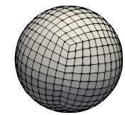 |
/blockMesh/sphere/
Creates the shown mesh using blockMesh.
The domain is a perfect sphere.
|
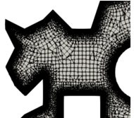 |
/foamyQuadMesh/jaggedBoundary/
Creates the shown mesh using foamyQuadMesh, which is explained in the User Guide as "Conformal-Voronoi 2D extruding automatic mesher
with grid or read initial points and point position relaxation with optional squarification". Whatever that is. Its name implies that it
creates 2D mehes with quadrilateral elements. So how do you learn what it really does? By studying these tutorial cases, searching on the
web and asking on user forums. This is what we mean by the steep learning curve.
The domain is a 2D jagged polygonal with holes in it. Only a part of it is shown here.
|
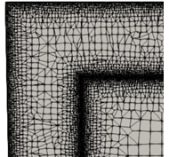 |
/foamyQuadMesh/square/
Creates the shown mesh again using foamyQuadMesh.
The domain is a 2D square with a square interface of fine cells. Only a part of it is shown here.
The 2D mesh is extruded into a wedge of 10 degrees to solve an axi-symmetric (not planar 2D) problem. Note that in OpenFOAM all problems
are actually set up as 3D. The trick to solve 2D problems is to limit the number of cells in the third dimension and provide special boundary
conditions.
|
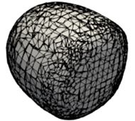 |
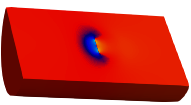
/foamyHexMesh/blob/
Creates the shown mesh using foamyHexMesh. This looks to be the 3D version of the foamyQuadMesh, creating hexahedral cells.
The domain is like a deformed sphere.
|
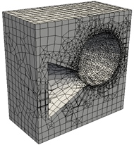 |
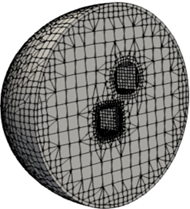
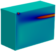
/foamyHexMesh/simpleShapes/
This is another case demonstrating the use of foamyHexMesh.
The domain is a cube with conical and shperical holes in it. Only half of it is shown here.
|
 |
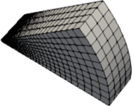
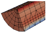
/foamyHexMesh/straightDuctImplicit/
And here is the third and the last foamyHexMesh tutorial.
The domain is a duct with square cross-section.
|
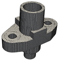 |
/snappyHexMesh/flange/
Creates the shown mesh using snappyHexMesh, which is an advanced mesher generating hexahedral dominant meshes, with split cells at the solid surfaces.
The domain is a 3D structural component.
|
 |
/snappyHexMesh/iglooWithFridges/
Another snappyHexMesh demonstration.
Semi-spherical domain has two holes in it.
|
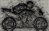 |
/snappyHexMesh/motorBike/
This is the third snappyHexMesh tutorial.
The domain is a rectangular box with a motor bike in it.
|
 |
/refineMesh/
Creates the shown mesh using blockMesh.
And performs adaptive mesh refinement (AMR).
|
4.2 Tutorials in the "basic" Folder
These problems are governed by simple PDEs, such as the Laplace's equation or the scalar transport equation.
 |
/laplacianFoam/flange/
Solves unsteady heat conduction over a flange, governed by the Laplace's equation.
|
 |
/potentialFoam/pitzDaily/
Solves the steady potential flow inside the 2D pitzDaily geometry, which is the classical backward facing step geometry
with an extra nozzle at the end.
|
 |
/potentialFoam/cylinder/
Solves the 2D, steady potential flow over a half cylinder.
Demonstrates the use of the function coding technique inside case files.
|
 |
/scalarTransportFoam/pitzDaily/
Solves the unsteady transport equation of a passive scalar inside the pitzDaily geometry with a known velocity
field.
|
4.3 Tutorials in the "incompressible/simpleFoam" Folder
simpleFoam is a steady, incompressible flow solver based on Spalding & Patankar's SIMPLE (Semi-Implicit Method for Pressure Linked Equations) algorithm.
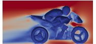 |
/motorBike/
20 m/s steady flow over a motorbike.
k-omega turbulence model is used.
|
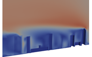 |
/windAroundBuildings/
10 m/s steady flow over buildings.
RANS type turbulence modeling is used.
|
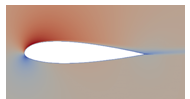 |
/airfoil2D/
26 m/s steady flow over a 2D airfoil at 8 degree angle of attack.
RANS type turbulence modeling is used with a wall function.
|
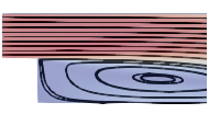 |
/pitzDaily/
10 m/s steady flow over the 2D pitzDaily geometry, which is a backward facing step with a nozzle at the end.
RANS type turbulence modeling is used.
Streamlines at the inlet and in the circulation zone are shown.
|
 |
/pitzDailyExpInlet/
Similar to the previous one, but this one uses the experimental data at the inlet.
Uses streamLine function object to generate streamline data.
Shown is the animation of the u velocity component through iterations.
|
 |
/mixerVessel2D/
2D simulation with fixed stators and rotating rotors.
A steady solution with multiple reference frame (MRF) technique is done.
Animation shows the variation of the flow field within the iterations of the steady solution.
|
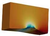 |
/turbineSitting/
Turbulent flow over a 3D terrain where wind turbines are to be installed.
Realistic atmospheric velocity profile at the inlet is specified.
Mesh generation and solution are both done using multiple processors.
|
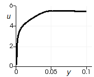 |
/T3A/
This is ERCOFTAC T3A 3% test-case, which is about the effect of inlet turbulence to transition over a flat plate.
Re is about half a million. k-omega SST model is used.
Shown is the velocity profile of the turbulent boundary layer at the end of the plate.
|
 |
/pipeCyclic/
Steady turbulent (Realizable k-epsilon) solution of flow inside a quarter pipe with periodic boundary conditions.
Adaptive mesh refinement is performed.
|
 |
/roomResidenceTime/
3D, turbulent flow is solved inside a room, with one inlet and one exit.
An extra transport equation is solved to determine the time taken for a particle to convect from the inlet to a
location in the flow.
Results are compared with experiments.
|
 |
/rotorDisk/
A 3 -bladed rotating disk is added into a cylindrical domain as a source, without actually modeling it in 3D.
Demonstrates the use of the "source" concept in OpenFOAM.
|
4.4 Tutorials in the "incompressible/pisoFoam" Folder
pisoFoam is an incompressible, transient flow solver based on Issa'a PISO (Pressure-Implicit with Splitting of Operators) algorithm.
 |
/laminar/porousBlockage/
A porous blockage is located inside a 2D duct as a source using the Darcy-Forchheimer law.
|
 |
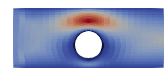
/ras/cavity/
2D lid-driven cavity problem is solved at Re = 0.5 million using the k-epsilon model.
Shown is the development of the pressure field during the transient solution.
|
 |
/les/pitzDaily/
Large Eddy Simulation of turbulent flow inside the pitzDaily benchmark geometry.
Demonstrates how to obtain mean variables from fluctuating ones.
Shown is the time varying velocity magnitude field.
|
4.5 Tutorials in the "incompressible/pimpleFoam" Folder
pimpleFoam is an incompressible, transient flow solver based on the combination of SIMPLE and PISO algorithms.
 |
/laminar/blockedChannel/
A porous blockage is located inside a 2D duct as a "source", based on the Darcy-Forchheimer law.
|
 |
/laminar/movingCone
A body is moving in the flow field.
Demonstrates how to handle moving boundaries and mesh deformation.
|
 |
/laminar/offsetCylinder
Demonstrates the use of a non-Newtonian fluid of power law type.
|
 |
/laminar/planarPoiseuille
Pressure driven Poiseuille flow inside a duct.
Uses a Maxwell type viscoelastic fluid.
Demonstrates the use of "momentum source" in the flow field.
Demonstrates how to probe the unsteady solution at a point.
planarCouette and planarContraction cases also demonstrate the use of viscoelastic fluids.
|
 |
/laminar/mixerVesselAMI2D
Similar to the mixerVessel case solved before using the steady simpleFoam solver, but this one is unsteady.
Demonstrates the use of Arbitrary Mesh Interface(AMI) capability. Here it is used to create a sliding mesh
interface between zones including rotors and stators.
|
 |
/laminar/pitzDailyPulse
Unsteady solution in the pitzDaily geometry.
Inlet velocity is defined as a cosine function.
Uses adaptive time step size with a maximum Courant number of 5.
|
 |
/RAS/Tjunction
Turbulent flow inside a T junction with one inlet and two outlets.
Probing is done at several points during the solution.
|
 |
/RAS/wingMotion2D
....
....
|
 |
/RAS/elipsekkLOmega
Flow over an elliptical body is solved using the kkL-omega model.
Mesh mirroring in both horizontal and vertical directions is applied.
|
 |
/RAS/propeller
....
....
|
 |
/RAS/...
....
....
|
| |
/RAS/...
....
....
|
 |
/LES/channel395
Large eddy simulation of channel flow with WALE (Wall-Adapting Local Eddy Viscosity) model.
Uses a momentum source of meanVelocityForce type to drive the flow.
Cyclic type boundary condition are used for inlet/outlet and front/back boundaries.
Seen here are the turbulent fluctuations of velocity magnitude.
|
< Previous Lecture TOC Next Lecture >