EasyNumerics Software

Home        Download & Installation        Screen Shots        Movies        Help        FAQ


How To Use The Software

Optimization

When you select the "Optimization" module from the main menu, the following window appears.


This module can be used to solve one-dimensional unconstrained optimization problems, using the following methods

  - Golden (and Arbitrary) Section Search
  - Quadratic Interpolation
  - Newton's Method

Golden Section Search is a bracketing method. It requires a function, two initial points (x0 < x1) that bracket only one optimum point (either a maximum or a minimum point) and whether the problem is a minimization or a maximization problem. Arbitrary Section Search is a generalized version of Golden Section Search and instead of the Golden Ratio, it uses any ratio in the range [0.5, 1]. Quadratic Interpolation is also a bracketing method but it requires three starting points (x0 < x1 < x2). Newton's Method is the classical Newton-Raphson method applied to the derivative of the function. It requires the first and second derivatives of the function and only one starting point.

After selecting a method and providing the required inputs, the solution can be started by pressing the Start button. If there is any missing entry, a warning message will appear at the output window. Otherwise some information about the selected parameters will be displayed. One can proceed with one iteration at a time or can complete all iterations at once. Details of the solution will be displayed at the output window. For the choice of one iteration at a time, the solution can be visualized at the Function Plot window with the help of auxiliarly lines and points. For the Quadratic Interpolation method the second order polynomial, and for the Newton's method the first derivative of the function will be displayed in gray. At the same time, the convergence plot can be watched at the Error Plot window. True errors will be calculated if the exact solution is specified. This plot is useful to compare convergnce characteristics of different solutions. For example one can perform several solutions using the Arbitrary Section Search method with different R values can compare their convergence.

To help understanding how to use this module, some snapshots taken during a sample run are shown below.

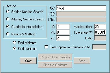
The first snapshot shows the entries. We will find the first positive optimum point of sin(x) (which is p/2) using the Quadratic Interpolation method. Starting points are specified as  x0=-1, x1=0, x2=2 . Note that the interval [x0, x1] must contain only one optimum point and x2 must be in this interval. Maximum number of iterations is selected to be 20 and the tolerance is set  to be 10-4. We also tell the program that we are afer a maximum point.

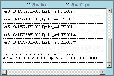
Second snapshot shows the Output window, which lists the final answer and the results of the final iterations. It took 7 iterations for the Quadratic Interpolation method to converge. Approximate relative errors are calculated at each iteration.

Third snapshot shows the Function Plot window after the first iteration. The black line is the function provided, sin(x). Three black points are the function values at the initial points provided by the user. Gray line is the parabola passing through these three points, and the red point is the maximum of this parabola. Red point is the estimated maximum after the first iteration.

Fourth snapshot shows the Function Plot window after the second iteration. After the first iteration a check was performed and one of the black points (x0 in this case) is replaced with the red point (actually with a point corresponding to sin(xred)). Now a new parabola is passed through this new set of black points and its maximum is calculated. The new red point is our new estimation.

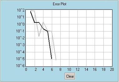
Fifth snapshot shows the Error Plot window. Gray line is the convergence based on the approximate relative errors (when the exact solution is not provided). Black line is the convergence based on the true relative errors (when the exact solution is provided) As seen approximate relative error plots generally have oscillatory behavior.


Please visit the movies section to watch sample runs of EasyNumerics.