|
How To Use The Software
Solving Systems of Linear Algebraic
Equations
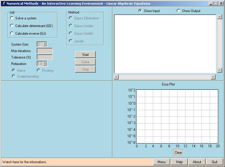
When you select the "Linear Algebraic Equations" module from
the main menu, the following window appears.

This module can be used for
- Solving a system of linear algebraic equations using the following
methods
- Gauss Elimination
- Gauss Jordan
- Gauss Seidel
- Jacobi
- Calculating the determinant of a system using Gauss Elimination
- Calculating the inverse and the condition number of a matrix using
Gauss-Jordan.
First you need to select the job from the top left window. If you want to solve
a system of equations you also need to select a method.
For direct methods (Gauss Elimination and Gauss-Jordan) you need to select the
system size. Also if you want to use pivoting (only partial-pivoting is
implemented) or scaled-pivoting, you can check the appropriate boxes. Note that
in scaled-pivoting, scaled coefficients will be used only for pivoting
decisions. Original (unscaled) coefficients will be used in the calculations.
For iterative methods (Gaus-Seidel and Jacobi) you will be asked to provide
maximum number of iterations and a tolerance value. Approximate relative percent
errors for each unknown will be calculated after each iteration and the program
will stop if the tolerance criteria is satisfied. Maximum number of iterations
is used eliminate an infinite loop in case of a diverging solution. For
iterative methods you can also specifiy a relaxation parameter (weighting
factor). You can use underrelaxation (0<l<1)
to make a diverging solution convergent or you can use overrelaxation (1<l<2)
to speed up a converging solution.
For calculating a determinant or taking an inverse, direct methods are used and
similar inputs are required.
After selecting the job and the method, the top right input window can be used
to enter the the matrices and vectors. For solving a system with direct methods,
a coefficient matrix and a right-hand-side vector are required. These need to be
entered in augmented form. A sample entry is shown below for a 3x3 system
9 1 4 14
4 16 9 29
9 10 25 44
There are 3 rows and 4 columns. Each row is entered on a separate line. Entries
are separated by a single space (using multiple spaces or tabs will not work).
The right-hand-side vector for the above example is (42.4 21.8
55.0). To calculate a determinant or take an inverse you do not need to provide
the right-hand-side vector.
To solve a system using an iterative method, you need to specify another column
that will be used as the initial guesses. The above sample entry will be changed
to
9 1 4 14 0
4 16 9 29 0
9 10 25 44 0
where the initial guess vector is (0 0
0). Now we have 3 rows and 5 columns.
After providing all the necessary data, you can press the "Start" buton and some
information will be displayed at the output window. (Note that the input and
output windows are on top of each other and only one of them can be shown at a
time. You can switch between the two using the radio buttons. Make sure you
enter the coefficients in the correct window). If you did not provide all the
necessary data, an error message will warn you about this. Othrewise you are
ready to continue with the solution. Press the "Solve" button. All the solution
will be done at once.
If you are solving a system using a direct method all the details of the forward
elimination step will be shown. First a scale vector will be displayed if you
selected to use scaled-pivoting. This vector will be used for all pivoting
decisions. Than Step (1), forward elimination, will start. It has many substeps.
For example (1.1) is about eliminating the first unknown from the other
equations. If you are using pivoting, at the beginning of each substep, an
information will be displayed about the switched rows, if there are any. Than
the reduced system will be shown. At the end of the forward elimination,
Gauss-Elimination method will result in an upper triangular system and
Gauss-Jordan will result in an identity matrix. Next step is the
backsubstitution, which is only necessary for Gauss-Elimination. Finally the
solution vector will be displayed. If you are working with a singular system, a
division by zero may occur at the last substep of forward elimination for
Gauss-Jordan and at the back substitution step for Gauss Elimination.
If you are using an iterative method, first the initial guesses is shown. Than,
after each iteration, new solutions and approximate relative percent errors for
all the unknowns are displayed. Iterations are stoped when either the tolerance
criteria is satisfied for all unknowns or the maximum number of iterations is
reached. A convergence graph is also generated for iterative solutions. It shows
the maximum relative persent error at each iteration. You can use this to
compare the convergence rates of Gauss-Seidel and Jacobi methods. Also the
affect of the relaxation can be seen clearly from this plot. Note that the error
plot is not cleared automatically so that you can put multiple graphs on top of
each other for comparison purposes. You can manually erase the error plot by
pressing the Clear button.
The output for calculating the deteminant or the inverse of a matrix is similar
to the outputs described for solving a system with direct methods.
After completing a solution you can modify the input data and solve another
system.
To help understanding the solution of linear
algebraic systems,
some snapshots taken during the calculation of the following system are shown below.
9x1 + x2 + 4x3
= 14
4x1 + 16x2 + 9x3 = 29
9x1 + 10x2 + 25x3 = 44
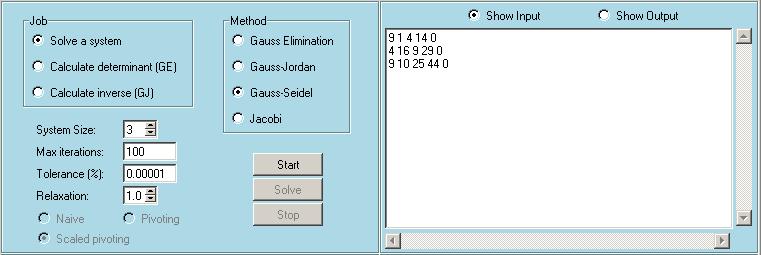
The first snapshot shows the entries. We will solve
a 3x3 system using the iterative Gauss-Seidel method. Maximum number of
iterations is selected to be 100, tolerance is set to be 10-5
and relaxation parameter is given as 1.0. The augmented coefficient matrix, the
right hand side vector and the initial guess vector is provided in the Input
window. the last column shows the initial guess vecto, which is (0, 0, 0). Note
that the exact solution of this system is (1, 1, 1).
Second snapshot shows the Output window, which lists
the results of the last three iterations (You can scroll up to see details of
the previous iterations). It took 15 iterations for Gauss-Seidel to converge
within the specified tolerance level. Approximate relative errors are calculated
at each iteration for all unknowns.
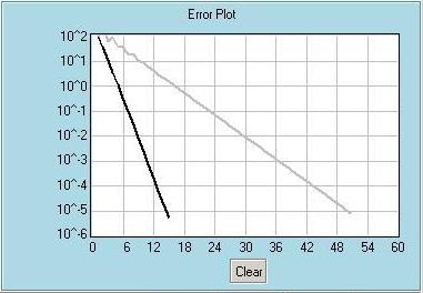
Third snapshot shows the relative errors plotted in
the Error Plot window. The black line is the convergence plot of the
Gauss-Seidel solution which took 15 iterations. The gray line is obtained from a
previous run, which solved the same problem using the Jacobi method. Jacobi
method took 51 iterations to reach the same error level. Error Plot window is
useful to make such comparisons.


Please visit the movies
section to watch sample runs of EasyNumerics. |
