|
EasyNumerics Software |
|
Curve Fitting
When you select the "Curve Fitting" module from the main menu, the following window appears.
The user first selects the type of curve fitting to be performed, either regression or interpolation. For regression, a model equation should be selected. It can be linear, exponential, power or saturation-growth-rate equation or a general nth degree polynomial. The result of the regression will be the constants A and B of these equations (or the coefficients of the polynomial in case of a polynomial fit). Then the number of data points is specified. If there is a point that you want to interpolate at, you can specify it. The data points should be entered in the Input Window. A sample of 5 input points is shown below
1.0 0.5 where the first and second columns are for the x and y values, respectively. There should be only a single blank character (no tabs) between x and y values. The data points and the equation found after the regression will be shown at the Function Plot window. If you select a point at which you want to interpolate, this point and the value of the interpolation will also be plotted. For interpolation you have three choices. Polynomial interpolation can be done using Newton's Divided Difference Interpolating Polynomials or Lagrange Polynomials. If using Newton's Polynomials a finite divided difference table will be generated. The data points and the calculated polynomial will be plotted. For Lagrange Interpolation the interpolating polynomial is the sum of several special polynomials. All these polynomials and their sum will be plotted. In this version the output of Lagrange Interpolation does not provide enough detail. Spline interpolation can be done for orders of 1, 2 or 3. For the first-order case, the slopes of the straight lines joining the data points will be calculated. For the second-order case, a (3n)x(3n) sytem will be solved with Gauss Elimination (with scaled pivoting) and the three constants of each spline will be shown. For the third-order case, an (n-1)x(n-1) system is solved for the second derivatives at the interior points. The data points and the splines will be plotted at the Function Plot window. Note that for spline interpolation, the data points should be entered in ascending order (from the lowest x to the highest x). In any type of interpolation, if the data points are obtained using a function, that function can be specified to calculate the true errors at the interpolation points. This function will also be plotted on top of the interpolating polynomial. To help understanding the details of regression, some snapshots taken during a a power equation fit for 5 data points are shown below.
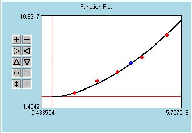
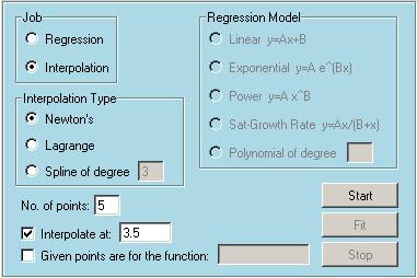
The first snapshot shows the entries. We want to perform a regression using the power equation for 5 points. We also want to interpolate at x=3.5. Second snapshot shows the Input Window, where we give the x and y values of the data points. Third snapshot shows the Output Window, which has the results after the regression. Many details like, sum of x values, mean of the x values, etc. used in the calculations are given. Sr is the sum of the squares of the residuals between the given and fitted y values. St is the sum of the squares of the residuals between the given y values and the mean. r2 is the coefficient of determination and r is the correlation coefficient. a0 and a1 are the coefficients appearing in the normal equations used for the linear least squares regression. A and B are the constants that needs to be determined in the selected power equation. Finally the result of the interpolation at point 3.5 is shown. Fourth snapshot shows the Function Plot window. Red points are the given data points. Black line shows the calculated power equation. Blue point, corresponding to x=3.5, is the interpolation point that we selected at the beginning. Now we will give the snapshots of a sample interpolation run.
The first snapshot shows the entries. We want to perform an interpolation using Newton's Interpolating polynomials with data 5 points. After the interpolation we will calculate the value at x=3.5. Second snapshot shows the Input Window, where we give the x and y values of the data points. We are using the same values as we used for the previous regression example. Third snapshot shows the Output Window. It basically has the Finite divided difference table. First and second columns are the provided x and y values. Remaining four columns are the calculated values (To see the last column you have to scroll to the right). The coefficients of the fourth order interpolating polynomial are obtained from the first row as 0.5, 1.6, -0.14035, 0.12759 and -0.017682. The value of the interpolating polynomial at x=3.5 is also calculated. Fourth snapshot shows the Function Plot window. Red points are the specifide data points. Black line shows the interpolating polynomial which exactly passes through all data points. Blue point corresponds to the specified x=3.5. Please visit the movies section to watch sample runs of EasyNumerics. |


