MATH382: LAB 3: Interpolation on evenly-spaced Points
This lab is
concerned with interpolating data with polynomials and with trigonometric
functions. There is a difference between interpolating and approximating.
Interpolating means that the function passes through all the given
points with no regard to the points between them. Approximating means that the
function is close to all the given points and probably close to nearby points
as well. It might seem that interpolating is always better than approximating,
but there are many situations in which approximation is the better choice.
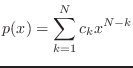
Polynomials
are commonly used to interpolate data. There are several methods for defining,
constructing, and evaluating the polynomial of a given degree that passes
through data values. One common way is to solve for the coefficients of the
polynomial by setting up a linear system called Vandermonde's equation.
A second way is to represent the polynomial as the sum of simple Lagrange
polynomials. Other ways are available and are discussed in the text and the
lectures. In addition, we will discuss interpolation using trigonometric
polynomials.
We will
examine these two ways of finding the interpolating polynomial and a way of
finding the interpolating trigonometric polynomial. We will see examples
showing that interpolation does not necessarily mean good approximation and
that one way that a polynomial interpolant can fail to approximate. Trigonometric
polynomial interpolation does better, but can also break down.
This lab is
focussed on finding functions that pass through certain specified points. In
customary notation, you are given a set of points ![]() and you want to find a function
and you want to find a function ![]() that
passes through each point (
that
passes through each point ( ![]() for
for
![]() ).
That is, for each of the abscissæ,
).
That is, for each of the abscissæ, ![]() ,
the function value
,
the function value ![]() agrees
with the ordinate
agrees
with the ordinate ![]() .
The given points are variously called the ``given'' points, the ``specified''
points, the ``data'' points, etc. In this lab, we will use the term
``data points.''
.
The given points are variously called the ``given'' points, the ``specified''
points, the ``data'' points, etc. In this lab, we will use the term
``data points.''
Written in
the customary notation, it is easy to see that the quantities ![]() and
and
![]() are
essentially different. In Matlab, without kerning and font differentiation, it
can be difficult to keep the various quantities straight. In this lab, we will
use the name xval to denote
the values of
are
essentially different. In Matlab, without kerning and font differentiation, it
can be difficult to keep the various quantities straight. In this lab, we will
use the name xval to denote
the values of ![]() and
the names xdata and ydata to denote the data
and
the names xdata and ydata to denote the data ![]() and
and
![]() .
The variable names fval or yval are used
for the value
.
The variable names fval or yval are used
for the value ![]() to
emphasize that it is an interpolated value.
to
emphasize that it is an interpolated value.
At some
point in this lab, you will need to determine if a quantity A is not equal to a quantity B. The Matlab syntax for this is
if A ~= B
Sometimes it
is convenient to enclose the logical expression in parentheses, but this is not
required.
If you have
a (square) linear system of equations, of the form
A * x = b
where A is an N by N matrix, and b and x are column vectors, then Matlab can solve the linear system either
by using the expression:
x = inv(A)*b
or, better,
via the ``backslash'' command:
x = A \ b
that you
used in the previous labs. The backslash command is strange looking. You might
remember it by noting that the matrix A appears underneath the backslash. The backslash is
used because matrix multiplication is not commutative, so a square matrix
should appear to the left of a column vector. The difference between the two
commands is merely that the backslash command is about three times faster
because it solves the equation without constructing the inverse matrix. You
will not notice a difference in this lab, but you might see one later if you
use Matlab for more complicated projects.
The
backslash command is actually more general than just multiplication by the
inverse. It can find solutions when the matrix A is singular or when it is not a square matrix! We
will discuss how it does these things later in the course, but for now, be very
careful when you use the backslash operator because it can find ``solutions''
when you do not expect a solution.
Matlab has
several commands for dealing with polynomials:
c=poly(r)
Finds the coefficients of the
polynomial whose roots are given by the vector r.
r=roots(c)
Finds the roots of the polynomial
whose coefficients are given by the vector c.
c=polyfit( xdata, ydata, n)
Finds the coefficients of the
polynomial of degree n passing through, or approaching as closely as possible, the points xdata(k),ydata(k), for ![]() ,
where
,
where ![]() need
not be the same as n.
need
not be the same as n.
yval=polyval( c, xval)
Evaluates a polynomial with
coefficients given by the vector c at the values xval(k) for ![]() for
for
![]() .
.
When there
are more data values than the minimum, the polyfit function returns the coefficients
of a polynomial that ``best fits'' the given values in the sense of least
squares. This polynomial approximates, but does not necessarily interpolate,
the data. In this lab, you will be writing m-files with functions similar to polyfit but that generate polynomials of
the precise degree determined by the number of data points. (n=length(xdata)-1).
The vector
of coefficients c of a
polynomial in Matlab are, by convention, defined as
Beware: When
a vector of numbers, c, of length N, is
regarded as coefficients of a polynomial of degree N-1, the subscripts run backwards! c(1) is the coefficient of the term with
degree N-1, and the
constant term is c(N).
In this and
some later labs, you will be writing m-files with functions analogous to polyfit and polyval, using several different methods.
Rather than following the matlab naming convention, functions with the prefix coef_ will generate a vector of
coefficients, as by polyfit, and functions with the prefix eval_ will evaluate a polynomial (or
other function) at values of xval, as with polyval.
In the this
lab and often in later labs we will be using Matlab functions to construct a
known polynomial and using it to generate ``data'' values. Then we use our
interpolation functions to recover the original, known, polynomial. This
strategy is a powerful tool for illustrative and debugging purposes, but
practical use of interpolation starts from arbitrary data, not contrived data.
The Polynomial through Given Data
Vandermonde's Equation
Here's one
way to see how to organize the computation of the polynomial that passes
through a set of data.
Suppose we
wanted to determine the linear polynomial ![]() that
passes through the data points
that
passes through the data points ![]() and
and
![]() .
We simply have to solve a set of linear equations for
.
We simply have to solve a set of linear equations for ![]() and
and
![]() .
.
|
|
|
|
|
|
|
|
or,
equivalently,
![$\displaystyle \left[\begin{array}{cc}x_1 & 1 x_2 & 1\end{array}\right]
\left[...
...c_1 c_2\end{array}\right]=
\left[\begin{array}{c}y_1 y_2\end{array}\right]
$](MATH382Lab4_files/image024.gif)
which
(usually) has the solution
|
|
|
|
|
|
|
|
|
|
Compare that
situation with the case where we want to determine the quadratic polynomial ![]() that passes through three sets of
data values. Then we have to solve the following set of linear equations for
the polynomial coefficients c:
that passes through three sets of
data values. Then we have to solve the following set of linear equations for
the polynomial coefficients c:
![$\displaystyle \left[\begin{array}{ccc}x_1^2 & x_1 & 1 [3pt]
x_2^2 & x_2 & 1\...
...c_3\end{array}\right]=
\left[\begin{array}{c}y_1 y_2 y_3\end{array}\right]
$](MATH382Lab4_files/image029.gif)
This is an
example of a third order Vandermonde Equation. It is characterized by
the fact that for each row (sometimes column) of the coefficient matrix, the
succesive entries are generated by a decreasing (sometimes increasing) set of
powers of a set of variables.
You should
be able to see that, for any collection of abscissæ and ordinates, it is
possible to define a linear system that should be satisfied by the (unknown)
polynomial coefficients. If we can solve the system, and solve it accurately,
then that is one way to determine the interpolating polynomial.
Now, let's
see how to construct and solve the Vandermonde equation using Matlab. This
involves setting up the coefficient matrix A. We use the Matlab variables xdata and ydata to represent the quantities ![]() and
and
![]() ,
and we will assume them to be row vectors of length n.
,
and we will assume them to be row vectors of length n.
for j = 1:n
for k = 1:n
A(j,k) =
xdata(j)^(n-k) ;
end
end
Then we have
to set the right hand side to the ordinates ydata, that is assumed to be a row vector. If we can get
all of that set up, then actually solving the linear system is easy. We just
write:
c = A \ ydata';
Recall that
the backslash symbol means to solve the system with matrix A and right side ydata'. Notice that ydata' is the transpose of the row vector ydata in this equation. (By default,
Matlab constructs row vectors unless told to do otherwise.)
Exercise 1: The Matlab
built-in function polyfit finds the
coefficients of a polynomial through a set of points. We will write our own
using the Vandermonde matrix. (This is the way that the Matlab function polyfit works.)
1. Write a Matlab function m-file, coef_vander.m with signature
2. function c = coef_vander ( xdata, ydata )
3. % c = coef_vander ( xdata, ydata )
4. % xdata= ???
5. % ydata= ???
6. % c= ???
7. % other comments
8.
9. % your name and the date
that accepts a pair of row vectors xdata and ydata of arbitrary but equal length, and returns the
coefficient vector c of the polynomial that passes through that data. Be sure to complete the
comments with question marks in them.
Warning: Think carefully about what to use for n.
10. Test your function by computing the
coefficients of the polynomial through the following data points. (This polynomial
is ![]() ,
so you can check your coefficient vector ``by inspection.'')
,
so you can check your coefficient vector ``by inspection.'')
11.xdata= [ 0 1 2
]
12.ydata= [ 0 1 4
]
13. Test your function by computing the
coefficients of the polynomial that passes through the following points
14.xdata= [
-3 -2 -1 0 1 2
3]
15.ydata= [1636 247 28
7 4 31
412]
16. Confirm using polyval that your polynomial passes through
these data points.
17. Double-check your work by comparing
with results from the Matlab polyfit function. Please include both the full polyfit
command you used and the coefficient vector it returned in your summary.
In the
following exercise you will construct a polynomial using coef_vander to interpolate data points and then
you will see what happens between the interpolation points.
1. Consider the polynomial whose roots
are r=[-3 -2 -1 1 2]. Use the
Matlab poly function to
find its coefficients. Call these coefficients cTrue.
2. This polynomial obviously passes
through zero at each of these five ``data'' points. We want to see if our coef_vander function can reproduce it. To use
our coef_vander function,
we need a sixth point. You can ``read off'' the value of the polynomial at x=0 from its coefficients above. What
is this value?
3. Use the coef_vander function to find the coefficients
of the polynomial passing through the ``data'' points
4. xdata=[ -3 -2
-1 0 1 2 ];
5. ydata=[ 0
0 0 ?? 0 0 ];
Call these coefficients cVander.
6. What coefficients would result from
using only the five roots as xdata? Explain.
7. Use the following code to compute
and plot the values of the two polynomials on the interval [0,5]. If you look
at the last line of the code, you will see an estimate of the difference
between the two curves. How big is this difference? (We will be using
essentially this same code in several following exercises. You should be sure
you understand what it does. You might want to copy it to a script m-file.)
8. xval=linspace(-3,2,4001); % test abscissae for plotting
9. yvalTrue=polyval(cTrue,xval); % true ordinates
10.yvalVander=polyval(cVander,xval); % our ordinates
11.plot(xval,yvalTrue,'b'); % true curve in blue
12.hold on
13.plot(xval,yvalVander,'r'); % our curve in red
14.hold off
15.max(abs((yvalTrue-yvalVander)))
Please include a copy of this plot with your summary.
(If it appears that there is only one curve, it is possible that the red curve
covers the blue one.)
Suppose we
fix the set of ![]() distinct
abscissæ
distinct
abscissæ ![]() ,
,
![]() and
think about the problem of constructing a polynomial that has (not yet
specified) values
and
think about the problem of constructing a polynomial that has (not yet
specified) values ![]() at
these points. Now suppose I have a polynomial
at
these points. Now suppose I have a polynomial ![]() whose
value is zero at each
whose
value is zero at each ![]() ,
,
![]() ,
and is 1 at
,
and is 1 at ![]() .
Then the intermediate polynomial
.
Then the intermediate polynomial ![]() would
have the value
would
have the value ![]() at
at
![]() ,
and be 0 at all the other
,
and be 0 at all the other ![]() .
Doing the same for each abscissa and adding the intermediate polynomials
together results in the polynomial that interpolates the data without solving
any equations!
.
Doing the same for each abscissa and adding the intermediate polynomials
together results in the polynomial that interpolates the data without solving
any equations!
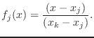
In fact, the
Lagrange polynomials ![]() are
easily constructed for any set of abscissae. Each Lagrange polynomial will be
of degree
are
easily constructed for any set of abscissae. Each Lagrange polynomial will be
of degree ![]() .
There will be
.
There will be ![]() Lagrange
polynomials, one per abscissa, and the
Lagrange
polynomials, one per abscissa, and the ![]() polynomial
polynomial
![]() will
have a special relationship with the abscissa
will
have a special relationship with the abscissa ![]() ,
namely, it will be 1 there, and 0 at the other abscissæ.
,
namely, it will be 1 there, and 0 at the other abscissæ.
In terms of
Lagrange polynomials, then, the interpolating polynomial has the form:

Assuming we can determine these magical polynomials, this is a second
way to define the interpolating polynomial to a set of data.
Remark: The strategy of finding a function
that equals 1 at a distinguished point and zero at all other points in a set is
very powerful. If ![]() in
(2),
then
in
(2),
then ![]() ,
so the
,
so the ![]() are
an example of a ``partition of unity.'' One of the places you will meet it
again is when you study the construction of finite elements for solving partial
differential equations.
are
an example of a ``partition of unity.'' One of the places you will meet it
again is when you study the construction of finite elements for solving partial
differential equations.
In the next
two exercises, you will be constructing polynomials through the same points as
in the previous exercise. Since there is only one nontrivial polynomial of
degree (n-1) through n data points, the resulting interpolating polynomials are
the same in these and the previous exercise.
In the next
exercise, you will construct the Lagrange polynomials associated with the data
points, and in the following exercise you will use these Lagrange polynomials
to construct the interpolating polynomial.
Exercise 3: In this
exercise you will construct Lagrange polynomials based on given data points.
Recall the data set for ![]() :
:
k : 1
2 3
xdata= [ 0 1
2 ]
ydata= [ 0 1
4 ]
(Actually, ydata is immaterial for construction of ![]() .)
In general, the formula for
.)
In general, the formula for ![]() can
be written as:
can
be written as:
(skipping the ![]() factor),
where each factor has the form
factor),
where each factor has the form
1. Write a Matlab function m-file
called lagrangep.m that
computes the Lagrange polynomials (3)
for any k. (One of
the Matlab toolboxes has a function named ``lagrange'', so this one is named ``lagrangep''.) The signature should be
2. function pval = lagrangep( k , xdata, xval )
3. % pval = lagrangep( k , xdata, xval )
4. % comments
5. % k= ???
6. % xdata= ???
7. % xval= ???
8. % pval= ???
9.
10.% your name and the date
and the function should evaluate the k-th Lagrange polynomial for the
abscissæ xdata at the
point xval. Hint, you
can implement the general formula using code like the following.
pval = 1;
for j = 1 : ???
if j ~= k
pval = pval
.* ??? % elementwise multiplication
end
end
Note: If xval is a vector of values, then pval will be the vector of corresponding
values, so that an elementwise multiplication (.*) is being performed.
11. Look carefully at the definition of
the Lagrange polynomials. From the definition alone, determine the values of lagrangep(
1, xdata, xval for xval=xdata(1), xval=xdata(2) and xval=xdata(3).
12. Check Matlab results against yours.
Does lagrangep give the
correct values for lagrangep( 1, xdata, xdata)? For lagrangep( 2, xdata, xdata)? For lagrangep( 3, xdata, xdata)?
Exercise 4: The hard
part is done. Now we want to use your lagrangep routine as a helper for a second
replacement for polyfit-polyval pair, called eval_lag, that implements Equation (2).
Unlike coef_vander, the
coefficient vector of the polynomial does not need to be generated separately
because it is so easy, and that is why eval_lag both fits and evaluates the
Lagrange interpolating polynomial.
1. Write a Matlab function m-file
called eval_lag.m with the
signature
2. function yval = eval_lag ( xdata, ydata, xval )
3. % yval = eval_lag ( xdata, ydata, xval )
4. % comments
5.
6. % your name and the date
This function should take the data values xdata and ydata, and compute the value of the interpolating
polynomial at xval according
to (2),
using your lagrangep function
for the Lagrange polynomials. Be sure to include comments to that effect.
7. Test eval_lag on the simplest data set we have
been using.
8. k : 1
2 3
9. xdata= [ 0
1 2 ]
10. ydata= [ 0
1 4 ]
by evaluating it at xval=xdata. Of course, you should get ydata back.
11. Test your function by interpolating
the polynomial that passes through the following points, again by evaluating it
at xval=xdata.
12.xdata= [
-3 -2 -1 0
1 2 3]
13.ydata= [1636 247 28
7 4 31
412]
14. Repeat Exercise 2 using Lagrange
interpolation.
o Return to the polynomial constructed
in Exercise 2 with roots r=[-3 -2 -1 1 2]. and coefficients cTrue.
o Reconstruct (using polyval) or recall the ydata values associated with xdata=[-3 -2
-1 0 1 2].
o Compute the values of the Lagrange
interpolating polynomial at the same 4001 test points between -3 and 2. Call
these values yvalLag.
Interpolating a function that is not a polynomial
Interpolating
functions that are polynomials and using polynomials to do it is cheating a
little bit. You have seen that interpolating polynomials can result in
interpolants that are essentially identical to the original polynomial. Results
can be much less satisfying when polynomials are used to interpolate functions
that are not themselves polynomials. At the interpolation points, the function
and its interpolant agree exactly, so we want to examine the behavior between
the interpolation points. In the following exercise, you will see that some
non-polynomial functions can be interpolated quite well, and in the subsequent
exercise you will see one that cannot be interpolated well.
Exercise 5: In this
exercise you will construct interpolants for the function ![]() and
see that it and its polynomial interpolant are quite close.
and
see that it and its polynomial interpolant are quite close.
1. We would like to interpolate the
function ![]() on
the interval
on
the interval ![]() ,
so use the following outline to examine the behavior of the polynomial
interpolant to the exponential function for five evenly-spaced points. It would
be best if you put these commands into a script m-file named exer5.m.
,
so use the following outline to examine the behavior of the polynomial
interpolant to the exponential function for five evenly-spaced points. It would
be best if you put these commands into a script m-file named exer5.m.
2. % construct n=5 data points
3. n=5;
4. xdata=linspace(-pi,pi,n);
5. ydata=exp(xdata);
6.
7. % construct many test points
8. xval=linspace(???,???,4001);
9. % construct the true function, for reference
10.yvalTrue=exp(???);
11.
12.% use Lagrange polynomial interpolation to evaluate
13.% the interpolant at the test points
14.yval=eval_lag(???,???,xval);
15.
16.% plot reference values in blue, interpolant in red
17.plot(xval,yvalTrue,'b');
18.hold on
19.plot(xval,yval,'r');
20.hold off
21.
22.% estimate the approximation error of the interpolant
23.approximationError=max(abs(yvalTrue-yval))
Please send me this plot.
24. By zooming, etc., confirm visually
that the exponential and its interpolant agree at the interpolation points.
25. Using more data points gives higher
degree interpolation polynomials. Fill in the following table using Lagrange
interpolation with increasing numbers of data points.
26. n = 5
Approximation Error = ________
27. n = 11 Approximation Error = ________
28. n = 21 Approximation Error = ________
You should
have observed in Exercise 5 that the approximation error becomes quite small.
The exponential function is entire, as are polynomials, so they share one
essential feature. In the following exercise, you will see that interpolating
functions that are not entire can give poor results.
1. Construct a function m-file for the
Runge example function ![]() .
Name the file runge.m and give it
the signature
.
Name the file runge.m and give it
the signature
2. function y=runge(x)
3. % y=runge(x)
4. % comments
5.
6. % your name and the date
Use componentwise (vector) division and exponentiation
(./ and .^).
7. Copy exer5.m to exer6.m and modify it to use the Runge
example function. Please send me the plot it generates.
8. Confirm visually that the Runge
example function and its interpolant agree at the interpolation points, but not
necessarily between them.
9. Using more data points gives higher
degree interpolation polynomials. Fill in the following table using Lagrange
interpolation with increasing numbers of data points.
10. n = 5
Approximation Error = ________
11. n = 11 Approximation Error = ________
12. n = 21 Approximation Error = ________
13. Are you surprised to see that the
errors do not decrease?
Most people
expect that an interpolating polynomial ![]() gives
a good approximation to the function
gives
a good approximation to the function ![]() everywhere,
no matter what function we choose. If the approximation is not good, we expect
it to get better if we increase the number of data points. These expectations
will be fulfilled only when the function does not exhibit some ``essentially
non-polynomial'' behavior. You will see why the Runge example function cannot
be approximated well by polynomials in the following exercise.
everywhere,
no matter what function we choose. If the approximation is not good, we expect
it to get better if we increase the number of data points. These expectations
will be fulfilled only when the function does not exhibit some ``essentially
non-polynomial'' behavior. You will see why the Runge example function cannot
be approximated well by polynomials in the following exercise.
Exercise 7: The Runge
example function has Taylor series
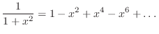
as you can easily prove. This series
has a radius of convergence of 1 in the complex plane. Polynomials, on the
other hand, are entire functions, i.e., their Taylor series' converge
everywhere in the complex plane. No finite sum of polynomials can be anything
but entire, but no entire function can interpolate the Runge example function
on a disk with radius larger than one about the origin in the complex plane. If
there were one, it would have to agree with the series (4)
inside the unit disk, but the series diverges at ![]() and
an entire function cannot have an infinite value.
and
an entire function cannot have an infinite value.
1. Make a copy of exer5.m called exer7.m that uses coef_vander and polyval to evaluate the interpolating
polynomial rather than eval_lag.
2. Confirm that you get the same
results as in Exercise 6 when you use Vandermonde interpolation for the Runge
example function.
3. n = 5
Approximation Error = ________
4. n = 11 Approximation Error = ________
5. n = 21 Approximation Error = ________
6. Look at the nontrivial coefficients
(![]() )
of the interpolating polynomials by filling in the following table.
)
of the interpolating polynomials by filling in the following table.
7. n=5 c( 5)=
_____ c( 3)= _____ c( 1)= _____
8. n=11 c(11)=
_____ c( 9)= _____ c( 7)= _____
c( 5)= _____
9. n=21 c(21)=
_____ c(19)= _____ c(17)= _____
c(15)= _____
10.limiting
+1 -1 +1 -1
11. Look at the trivial coefficients (![]() )
of the interpolating polynomials by filling in the following table. (Look
carefully at what the colon notation does.)
)
of the interpolating polynomials by filling in the following table. (Look
carefully at what the colon notation does.)
12.n=5
max(abs(c(2:2:end)))= _____
13.n=11
max(abs(c(2:2:end)))= _____
14.n=21
max(abs(c(2:2:end)))= _____
You should see that the
interpolating polynomials are ``trying'' to reproduce the Taylor series (4).
These polynomials cannot agree with the Taylor series at all points, though,
because the Taylor series does not converge at all points.
Trigonometric polynomial interpolation
Quarteroni,
Sacco, and Saleri discuss interpolation by trigonometric polynomials in Section
10.1. Trigonometric interpolation is closely related to approximation by
Fourier series, but we will focus on interpolation in this lab.
The basic
expression for trigonometric interpolation using ![]() functions
over the interval
functions
over the interval ![]() is
is
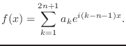
(We consider
![]() points
because we want to use real functions and real interpolants. Thus one
trigonometric function
points
because we want to use real functions and real interpolants. Thus one
trigonometric function ![]() is
the constant term when
is
the constant term when ![]() ,
and all the rest come in complex conjugate pairs.)
,
and all the rest come in complex conjugate pairs.)
Using the ![]() evenly-spaced
points in the interval
evenly-spaced
points in the interval ![]() given
by
given
by
the
coefficients can be determined from
These
equations can be found directly by multiplying (5)
through by each of the functions ![]() in
turn, applying it to the values
in
turn, applying it to the values ![]() ,
and solving the resulting system for
,
and solving the resulting system for ![]() ,
taking advantage of the properties of the complex exponential to simplify the
equations.
,
taking advantage of the properties of the complex exponential to simplify the
equations.
Remark: The trigonometric coefficients ![]() in
(7)
play the same role as the polynomial coefficients
in
(7)
play the same role as the polynomial coefficients ![]() in
(1).
in
(1).
In the
following exercises, we are going to write functions coef_trig to be analogous to polyfit and coef_vander, and also eval_trig to be analogous to polyval and eval_lag.
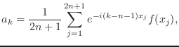
1. Construct a function m-file named coef_trig.m with the signature
2. function a=coef_trig(f,n)
3. % a=coef_trig(f,n)
4. % f=???
5. % n=???
6. % a=???
7. % comments
8.
9. % your name and the date
This function should evaluate the trigonometric
coefficients ![]() according
to Equation (7).
Use Equation (6)
to determine the points
according
to Equation (7).
Use Equation (6)
to determine the points ![]() .
It is more efficient to use vector (componentwise) notation and the Matlab sum function, but if you cannot see how
to do that, just use for loops.
.
It is more efficient to use vector (componentwise) notation and the Matlab sum function, but if you cannot see how
to do that, just use for loops.
Hint: You can use the following code to generate the
points ![]() without
writing a for loop.
without
writing a for loop.
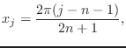
xdata = 2*pi*(-n:n)/(2*n+1);
Note: The length of a should be 2*n+1.
10. Test your function by applying it to
the function ![]() ,
for n=10. (You can either write an m-file for
,
for n=10. (You can either write an m-file for ![]() or
use Matlab's inline command. If
you are using a recent version of Matlab, you can use the @ command to define an ``anonymous
function.'') By examining Equation (5),
you should be able to see that
or
use Matlab's inline command. If
you are using a recent version of Matlab, you can use the @ command to define an ``anonymous
function.'') By examining Equation (5),
you should be able to see that ![]() for
for
![]() and
zero otherwise.
and
zero otherwise.
11. Test your function again by applying
it to ![]() with
n=10. You should
see that
with
n=10. You should
see that ![]() is
zero for all but two subscripts. What subscripts (
is
zero for all but two subscripts. What subscripts (![]() )
have non-zero
)
have non-zero ![]() and
what are the values?
and
what are the values?
1. Construct a function m-file named eval_trig.m with the signature
2. function fval=eval_trig(a,xval)
3. % fval=eval_trig(a,xval)
4. % a=???
5. % xval=???
6. % fval=???
7. % comments
8.
9. % your name and the date
This function should evaluate Equation (5)
at an arbitrary collection of points, xval.
10. Test your function by first using coef_trig to find the coefficients for the
function ![]() with
n=10 (you did
this in the previous exercise), and then applying eval_trig to those coefficients at 4001
equally-spaced points in the interval
with
n=10 (you did
this in the previous exercise), and then applying eval_trig to those coefficients at 4001
equally-spaced points in the interval ![]() .
Compare the interpolated values versus
.
Compare the interpolated values versus ![]() .
Plot them on the same plot: the lines should overlap. You can modify the m-file
exer5.m that you
wrote for Exercise 5. Call your modified m-file exer9.m. (Warning: Your interpolated values
may appear to Matlab to be complex, and Matlab may not plot them the way you
expect. In that case, verify that their imaginary parts (Matlab function imag) are zero and plot only the real
(Matlab function real) parts.
Please send me the plot.
.
Plot them on the same plot: the lines should overlap. You can modify the m-file
exer5.m that you
wrote for Exercise 5. Call your modified m-file exer9.m. (Warning: Your interpolated values
may appear to Matlab to be complex, and Matlab may not plot them the way you
expect. In that case, verify that their imaginary parts (Matlab function imag) are zero and plot only the real
(Matlab function real) parts.
Please send me the plot.
Trigonometric
polynomial interpolation does well even when the functions are not themselves
trigonometric polynomials.
1. Modify exer9.m to use the function ![]() ,
and call the modified file exer10.m. Plot the function and its interpolant for n=5, 10, 15 and n=20. You do not
have to send me the plots, but fill in the following table.
,
and call the modified file exer10.m. Plot the function and its interpolant for n=5, 10, 15 and n=20. You do not
have to send me the plots, but fill in the following table.
2. n = 5 x.*(pi^2-x.^2) Approximation Error =
________
3. n = 10
x.*(pi^2-x.^2) Approximation Error = ________
4. n = 15
x.*(pi^2-x.^2) Approximation Error = ________
5. n = 20
x.*(pi^2-x.^2) Approximation Error = ________
6. Do the same thing for the Runge
example function and fill in the following table.
7. n = 2 Runge Approximation Error = ________
8. n = 4 Runge Approximation Error = ________
9. n = 5 Runge Approximation Error = ________
You do not have to send me the plots.
10. For the n=2 case, and the Runge example
function, the five points at which the trigonometric interpolation should
interpolate the Runge example function are
11.xval=2*pi*(-2:2)/5;
Check that runge and eval_trig agree at those points.
The previous
exercise shows that trigonometric polynomial interpolation does well for some
functions. It does much less well when the function is not continuous or not
periodic in ![]() .
Consider, for example, the function
.
Consider, for example, the function
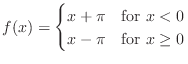
1. Copy the following code into a
function m-file named sawshape6.m
2. function y=sawshape6(x)
3. % y=sawshape6(x)
4. % x=???
5. % y=???
6. % comments
7.
8. % your name and the date
9.
10.kless=find(x<0);
11.kgreater=find(x>=0);
12.y(kless)=x(kless)+pi;
13.y(kgreater)=x(kgreater)-pi;
Be sure to add the usual comments.
14. The Matlab find command is a very useful function.
Use the help find command or
the Help facility to see what it does.
15. If x=[0 1 2 3 4 5 6 7 8 9 8 7 6], what is the result of the function
calls find(x==2), find(x==7), and find(x>5)?
16. Use a script file based on exer9.m to fill in the following table by
interpolating the sawshape6 function
using trigonometric interpolation.
17. n = 5
Approximation Error = ________
18. n = 10
Approximation Error = ________
19. n = 100 Approximation Error = ________
You can see that the approximation error is not
shrinking, but if you look at the plots you will see that the error really is
shrinking everywhere except near zero, where the oscillations get more rapid
but do not get smaller. This behavior is typical and is called Gibbs's
phenomenon. Please send me only the plot for n=100.
Increasing
the order of polynomial interpolation can lead to divergence of approximation
because of ``the wiggles.'' Trigonometric interpolation does not diverge as ![]() ,
but Gibbs phenomenon keeps the approximation from converging at
discontinuities.
,
but Gibbs phenomenon keeps the approximation from converging at
discontinuities.